Orbital Simulation Code
Gravitational and Atomic Models
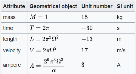
if we assign geometrical objects to mass, space and time at the Planck scale,
and then link them via this unit number relationship,
we can build a physical universe from pure mathematical structures.
Could a Programmer God have used this approach?
Gravitational and atomic orbital simulations based on the Planck-scale model described in Article 3 and Article 4 and referenced on the wiki-site are given here. The codes are written in C and python, C is faster and so better for long orbital radius and large center mass. I use codeblocks for my C compiler and Spyder for python but there are many online compilers. The codes here can be used under creative commons CC CC BY-NC-SA 4.0. This permits modifications to the code with attibution to the author.
This page assumes that the reader is already familiar with the article and/or wiki page. The following sections refer to different aspects (2-body orbits, elliptical orbits, transition orbits ...), but the orbital section routine in each case is the same. I have separated simply them to keep the code readable.
The model is designed to represent events at the Planck scale and so the mathematics is simple but computationally intensive. The core concept behind this approach is that the universe does not require an external set of commands, rather it could be a geometrically autonomous computer; electrons orbit protons, not because of an external function (a set of pre-programmed rules as with our simulations), but due to geometrical imperatives, the respective geometries of the electron and proton leading to these orbits. The incremental expansion of the universe does the rest (as it expands it pulls the particles with it).
Variables (2-body orbits):
ipoints: number of points in the central mass (the Scwharzchild radius)
jpoints: total number of points (in a 2-body orbit, the orbiting point is 1 mass unit; jpoints = ipoints +1)
kr: sets orbital radius as multiples of ipoints (quantizes radius as a function of the Scwharzchild radius)
x[0], y[0]: start coordinates for the orbiting point
x[1], y[1]: start coordinates for the orbited mass center point (some simulations have x[1], y[1] and x[2], y[2]).
The Kepler derivation in Maple code format.
Note: the simulation itself doesn't distingush between points, they all rotate around each other and so the points may also be assigned random co-ordinates for complex orbits. The 2-body orbit is however the most convenient for comparison with real-world orbits. Comments and suggestions are welcome, the code is not optimized, further improvements to the averaging and orbital stability can be added but these must reflect the geometrical autonomy of the model.
wiki- gravitational and atomic orbitals